CRITICAL LOAD DETERMINISTIC INTERVAL ESTIMATION FOR VARIABLE-STIFFNESS RODS USING THE INITIAL PARAMETER METHOD

This paper presents a modified initial parameter method for deterministic interval estimation of critical loads in axially compressed variable-stiffness rods. In the present study, the term “interval” refers to the range bounded by lower and upper estimates obtained from inscribed and circumscribed piecewise-constant geometric approximations of continuously varying cross-sections. The method approximates continuously varying cross-sections by inscribed and circumscribed piecewise-constant segments, providing reliable upper and lower bounds without requiring closed-form solutions. The formulation is applicable to both conservative and follower-load problems under various boundary conditions. Numerical examples for conical and smoothly varying rods demonstrate monotonic convergence of the estimates, with relative deviations below 1–3% for refined discretization. The proposed framework provides a computational tool for stability analysis of structural elements with variable stiffness and establishes rigorous deterministic lower and upper bounds that may serve as a baseline for subsequent uncertainty or reliability analyses. The present study is restricted to linear elastic rod theory; extension to elastoplastic behaviour is considered as a possible direction for future research.

1         Introduction

The stability of axially compressed rods and beam-like structures is a classical problem in structural mechanics and continues to attract significant interest due to its broad engineering applications. Fundamental theories of elastic stability, including both conservative and non-conservative formulations, were established in the pioneering works [1–6]. Among the analytical methods developed for such problems, the initial parameter method (IPM) has proven to be an efficient framework for vibration and stability analysis of rod systems by transforming governing differential equations into systems with piecewise-constant coefficients and transfer relations between state variables [7]. Its application has recently been extended to inhomogeneous and centrally compressed rods, demonstrating its effectiveness in solving more complex stability problems [8].

Recent research on critical load estimation has developed along several directions. Simplified computational models and substitution-based techniques have been proposed for evaluating buckling loads of cracked or complex structural elements [9–12]. Advanced formulations have also incorporated nonlinear effects, moment–rotation dependency, multiaxial loading, and shell stability problems, considerably expanding the scope of critical load analysis [13–18]. These studies provide effective computational tools, although they are generally aimed at direct numerical prediction rather than interval-type estimation.

At the same time, considerable attention has been devoted to structures with spatially varying stiffness. Previous studies have examined post-buckling behavior of elastic rods, variable-stiffness biomedical rods, adaptive rod systems, and constrained compression rods [19–22]. More recent work has addressed tapered and functionally graded beams, nanobeams, elastic curves with variable bending stiffness, and variable-stiffness composite shell structures [23–28]. In addition, studies of structurally inhomogeneous elastic elements and graded cylindrical shells have further demonstrated the important influence of spatial non-uniformity on stability characteristics [29,30]. However, despite these advances, most available approaches rely on differential equations with variable coefficients or standard discretization methods and do not provide guaranteed upper and lower bounds for critical loads.

This indicates the need for computationally efficient deterministic deterministic interval-based methods capable of producing rigorous lower and upper estimates for stability parameters in rods with variable stiffness. In the present work, the interval estimates are generated through inscribed and circumscribed piecewise approximations of continuously varying cross-sections rather than through probabilistic or stochastic uncertainty modeling. In particular, combining deterministic interval estimation with the initial parameter method for both conservative and non-conservative stability problems remain insufficiently explored.

In many modern engineering applications, including lightweight aerospace members, tapered composite structures, and slender adaptive systems, structures with strong geometric non-uniformity require reliable stability assessment. Although the present paper focuses on idealized conical and smoothly varying rods, these examples are intended as fundamental benchmark problems that establish the deterministic bounding framework necessary for future applications to more complex engineering structures. For such systems, manufacturing tolerances, local stiffness reduction, and continuously varying cross-sections may significantly influence stability behavior. In this context, rigorous deterministic lower and upper bounds for critical loads are of practical importance, since they provide a reliable baseline for subsequent uncertainty or reliability analyses without introducing probabilistic assumptions into the present formulation. Therefore, computational approaches capable of providing reliable lower and upper bounds for critical loads are of considerable practical interest.

The present study addresses this gap by developing a modified formulation of the initial parameter method for deterministic interval estimation of critical loads in axially compressed rods with variable stiffness. The proposed approach approximates continuously varying cross-sections by systems of inscribed and circumscribed piecewise-constant segments, enabling reliable bounds for critical loads without requiring closed-form solutions of differential equations with variable coefficients. Numerical examples demonstrate monotonic convergence and high accuracy of the proposed estimates, confirming the consistency and practical applicability of the proposed deterministic estimation procedure.

2         Materials and methods

2.1        Modification of the initial parameter method algorithm

A straight composite rod is defined as a rod whose stiffness and distributed mass are stepwise (piecewise-constant) functions of the longitudinal coordinate. According to the definition of a rod given in [5], these characteristics are assumed to be continuous and smooth functions of the longitudinal coordinate. Therefore, a composite rod may be regarded as a system of straight rods with constant stiffness, sharing a common straight axis; that is, the centroids of the cross-sections of the constituent rods lie on the same straight line.

For such unbranched rod systems, the simplest mathematical model can be constructed using the initial parameter method (IPM) [2]. In essence, this approach reduces solving the Cauchy problem for a system of ordinary differential equations with piecewise-constant coefficients. At points of first-kind discontinuity, continuity conditions of the solution are imposed: the state at the end of the preceding segment serves as the initial state for the subsequent segment. In terms of the IPM, this can be expressed as follows:

where $y_0$ is the state vector of the rod, i.e., a column vector composed of the nonzero state components of the rod (displacements, cross-sectional rotation angles, torsional and bending moments, axial and transverse forces); the superscript denotes the rod number; the subscript 0 refers to the initial state.

The matrix $B(x)$ is the normalized matrix of fundamental solutions of the differential equations of state, calculated at the point $0\le x\le L$, (L is the length of the rod). It is assumed that the equations of state allow the solution for one rod to be represented in the form

Representation (2) is applicable in both statics and dynamics when determining eigenstates; in this case, the unknown natural frequency of free oscillations, $\omega$, must be included among the arguments (all additional arguments are omitted for brevity). The boundary conditions at the beginning of the rod are satisfied by selecting a subset of the initial parameters, as follows, directly from the support conditions at the rod’s initial end. The remaining initial parameters are determined from the support conditions at the opposite end of the rod.

In the analysis of free vibrations, the boundary conditions are homogeneous; accordingly, the resulting system for determining the initial parameters is a homogeneous system of linear algebraic equations. The parameter ω is obtained from the condition that the principal determinant of this system vanishes, and the initial state vector is given by a nontrivial solution of the corresponding homogeneous system.

For a composite rod (1), the formula connecting the initial parameters with the state of the end of the rod is obvious:

Here, the product of the fundamental solution matrices should be interpreted as the influence matrix of the initial node of the rod system, numbered 0, on the terminal node, numbered N. The term “rod system” is used in the above-defined sense, with node numbering 0, ... , N and rod numbering 1, ... , N. Thus, for a single rod, there are nodes 0 and 1 and rod 1; the matrix $B_{01}$ represents the normalized fundamental solution matrix B(L)

Note that the fundamental solution matrix is computed in a local coordinate system whose origin is located at the initial end of the rod. The longitudinal axis is directed from the initial end to the terminal end, and the y- and x-axes coincide with the principal centroidal axes of inertia of the cross-section.

The IPM is applied to the problem of transverse vibrations of a composite rod. Within the framework of linear elastic material behavior and the Bernoulli hypothesis [5, 6], the differential state equation of a straight rod, accounting for the influence of the axial force on bending, has the form [3, 4]:

where $v$ is the transverse displacement; N is the axial force, assumed to be a known smooth and continuous function of the spatial coordinate and time; $\theta=v'$ is the angle of rotation of the cross-section; E and $\rho$ are Young’s modulus and the material density, respectively; A and J are the cross-sectional area and the principal centroidal moment of inertia; $q_y(x,t)$ is the distributed transverse load; t denotes time; (') indicates differentiation with respect to the longitudinal coordinate; and (.) denotes differentiation with respect to time.

At the rod ends, force boundary conditions may be prescribed:

or kinematic boundary conditions:

Mixed boundary conditions are also possible, defining admissible combinations of force and kinematic constraints. Note that the second term in the second and third equations represents the projection of the axial force onto the normal to the deformed axis at the initial or terminal end of the rod and is nonzero only in the case of a “dead” axial force directed along the undeformed axis of the rod. For a follower force, this term should be omitted, since a follower load is always directed tangentially to the axis in both the initial and deformed configurations.

The initial conditions are given by

Equation (4) is reduced to the following first-order system:

Even in the case of constant rod parameters, the coefficients of the last equation in system (8) depend on both the spatial coordinate and time. For the time being, the axial force is assumed to be independent of time, which makes it possible to apply separation of variables to Eqs. (4) and (8).

We reduce the system of state equations to dimensionless form by introducing the relative coordinate $\xi=\frac{\pi}{L}$ the dimensionless variables $\varpi=\frac{v}{L}; \theta; \mu=\frac{ML}{EJ}; \Theta=\frac{QL^2}{EJ}; n^2=\frac{NL^2}{EJ}$ as well as the dimensionless load parameters $\gamma_x=\frac{q_xL}{EA}; \gamma_y=\frac{q_yL^2}{EJ}$ and the frequency parameter $\Omega^4=\omega^2T^2=\frac{\omega^2\rho AL^4}{EJ}$ where $T^2=\frac{\rho AL^4}{EJ}$, and the dimensionless time $\tau=\frac{t}{T}$     

In these variables, the system of state equations takes the form $\psi'(\xi,\tau)=A\psi(\xi,\tau)-M\ddot{\psi}(\xi,\tau)+\gamma(\xi,\tau)$ where the state vector is defined as $\psi=\begin{pmatrix}\varpi\\\theta\\\mu\\\Theta\end{pmatrix}$ The system matrices and the external load vector are given by

9)

If the axial force is constant along the length, then $\frac{\partial}{\partial\xi}\left[n^2(\xi)\right]=0$ and the third coefficient in the last row of matrix A in (9) becomes constant. In this case, the solution of equation (9) can be readily obtained, for example, by applying the Laplace transform. Then, the nonzero components of the normalized fundamental solution matrix for the dynamic bending problem take the form

Using the modal expansion method [5] to solve the nonhomogeneous problem (9), let us consider the associated homogeneous problem obtained for $\gamma=0$. The solution of the homogeneous problem can be represented in the form

where $\Psi_0(\Omega)=(\varpi,\theta,\mu,\Theta)^T_{\xi=0}$     

Here, $\psi_0$ is the vector of initial state parameters, which has the meaning of amplitude functions under the assumption that the rod response can be expressed using the Fourier method in the form

The parameter $\omega$ represents the dimensionless natural frequency of free vibrations of the rod.

The boundary conditions (5), (6) in dimensionless form can be written as

Here, the subscript 0 denotes the components of the initial state vector, the subscript b refers to the external force factor applied at the left end of the rod, and the subscript e denotes the corresponding quantity at the right end.

When determining the spectrum, the dimensionless external forces and moments $\theta_e, \theta_b, \mu_e$, and $\mu_b$ should be taken equal to zero.

It should be noted that for rod systems, the dimensionless equations cannot be applied directly, since each rod possesses its own set of dimensionless variables and its own dimensionless time scale.

Therefore, when analysing rod systems (or composite rods), it is necessary to return to the dimensional formulation of the state variables. This can be accomplished by premultiplying the fundamental solution matrix by a constant diagonal matrix:

The introduction of dimensionless time is not practical; therefore, the physical time variable should be retained in the state equations. In this case, the analytical expressions (10) must be written in terms of the dimensional frequency instead of the dimensionless frequency $\Omega$. The relation between them is given by

Thus, for a system of rods, the transfer (influence) matrix can be written in the following form:

Here, $B_n$ denotes the fundamental solution matrix of the n-th rod evaluated at $\psi=1$, and $D_n$ are constant diagonal transformation matrices ensuring the transition between dimensional state vectors of adjacent rods.

The structure of the matrix product indicates that the procedure first involves the transformation from the dimensionless variables of the preceding rod segment to dimensional variables, and subsequently from dimensional variables to the dimensionless variables of the next segment.

Thus, the input to the system is represented by the dimensionless state variables of the initial segment, while the output corresponds to the dimensionless variables of the final segment:

Accordingly, the boundary conditions should be imposed in the form given in (13).

The proposed formulation is applicable to both continuously varying and discontinuous cross-sections, since compatibility conditions between adjacent segments are satisfied automatically within the transfer-matrix framework. The present study is limited to linear elastic rod theory. Extension of the proposed framework to elastoplastic problems through updated tangent stiffness formulations and incremental analysis is considered as a topic for future research.

2.2        Verification of the method

As an example of the application of the method, consider the problem of transverse free vibrations of a rod composed of three segments, as discussed in [4] (Fig. 1).

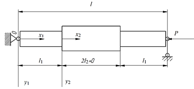
Fig. 1. Configuration of the rod [4]

The rod parameters were specified as follows: the material of the rod was steel with Young's modulus E= 200 GPa and density $\rho=7850\ kg/m^3$. The rod length was 1 m, and its cross-section was a solid circular section of diameter d. The geometric ratios were defined as $a=\beta l_1,\ 0<\beta\leq1, d_2=\lambda l_1$, and $d_1=\alpha d_2$. The parameter $\lambda$ was taken as 0.05 (i.e., the rod is slender), while the remaining parameters-the length ratio $\beta$ and the diameter ratio $\alpha$-were varied during the study.

First, the diameter ratio was taken as $\alpha=1$, i.e., the rod is uniform (smooth). The length ratio was varied within the range $\beta=0.2\ldots0.8$. The calculation results for all values were found to be identical; one example corresponding to $\beta=0.25\ (l_2=2l_1)$ is shown in Fig. 2. The vertical lines indicate the bifurcation points of a smooth pin-supported rod.
Figure 3 presents the results of determining the critical load for different geometric ratios of the rod (see Fig. 1).

For comparison of the results obtained (Fig. 3) with those reported by A. S. Volmir [4], they are expressed in terms of the dimensionless critical load K:

It should be noted that the definition of the parameter $\alpha$ in this paper differs from that in [4]: in the present study, $\alpha$ denotes the ratio of the diameters of sections 1 and 2, whereas in [4] it represents the ratio of the moments of inertia of the same sections. Therefore,

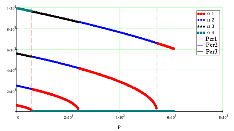
Fig. 2. Natural frequencies of the rod (Fig. 1) for equal diameters (P – compressive force, kN)

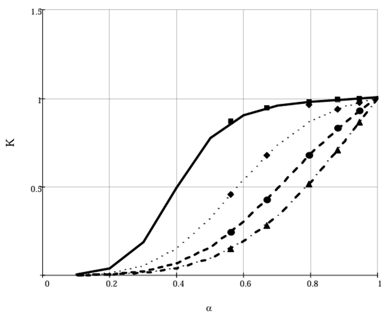
Fig. 3. Dependence of the dimensionless critical load K on the diameter ratio $\alpha=\frac{d_1}{d_2}$; solid line $\beta=0.8$, dotted line $\beta=0.6$, dashed line $\beta=0.4$, dash-dotted line $\beta=0.2$

From the figure presented, it can be seen that the results are consistent; however, the method of initial parameters is more universal with respect to the number of rod segments. Formula (16) applies to an arbitrary number of segments and is always reduced to a system of second-order equations, since the compatibility conditions at the interfaces between segments are satisfied automatically. Furthermore, the critical load is determined from the first discontinuity (jump) in the value of the first natural frequency (Fig. 3), i.e., within a dynamic formulation, which is important when solving nonconservative problems.  

3             Results and discussion

3.1        Critical load estimates for a conical rod

We consider problems demonstrating the capabilities of the method of initial parameters in determining critical loads within a dynamic formulation for composite rods with various ratios of segment lengths and stiffnesses.

Let the profile of the rod be bounded by a truncated cone with the maximum base diameter. $d_o$ and the minimum diameter $d_k$. We consider a sequence of problems arising in the approximation of the longitudinal section by cylinders inscribed in it and circumscribed about it (Fig.4).

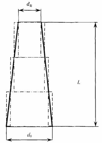
Fig. 4. Longitudinal section, inscribed and circumscribed cylinders, n=3

The lengths of all rods (segments) into which the original conical rod is divided are assumed to be equal. In this case, the diameters of the inscribed and circumscribed cylinders can be expressed as sequences:

Here, $\alpha$ denotes the semi-vertex angle of the cone, and n is the number of segments. The material of all segments is assumed to be identical: $E=2\cdot10^6$ MPa and $\rho=7850$  (steel, grade 3). The total length of the rod is L=1 m, and $\tan(\alpha)=0.2$. The first four natural frequencies were computed for various values of the compressive force in both conservative and nonconservative formulations (with a clamped base).

Figures 5 and 6 present estimates of the critical load for a conical rod, clamped at the larger-diameter end, under follower and “dead” loads, divided into five segments. In all figures, solid markers correspond to circumscribed cylinders (over), while open markers correspond to inscribed cylinders (inner). To refine the values of the critical load, the curves presented in Figs. 5, 6 were approximated by second-order parabolas using the least squares method.

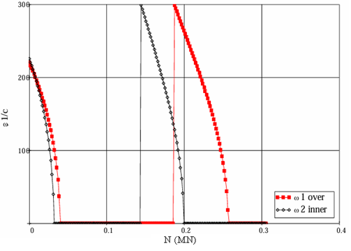
Fig. 5. Estimate of the critical load (five segments n=5, “dead” load)

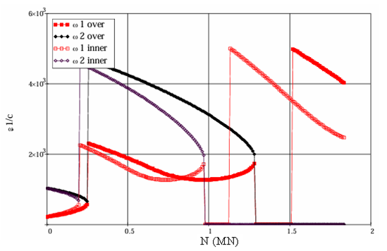
Fig. 6. Estimate of the critical load (five segments n=5, follower load)

For non-conservative problems, the approximation was constructed along both branches of the semi-loop in the form:

and the critical load was determined as the point of maximum:

For conservative problems, the approximation was performed along the descending branch of the parabola in the form:

and the critical load was determined as the positive root of the parabola:

The results of the estimation are presented in Table 1.

Table 1. Critical load estimation for a conical rod

The relative error $\delta$ was evaluated as the ratio of the difference between the upper $N_over$ and lower $N_inner$ estimates to their sum:

The results presented in the table show that, for a conical rod clamped at its base, the estimates obtained using the systems of circumscribed and inscribed cylinders converge; moreover, within the considered numbers of partitions, the convergence is monotonic. This fact indicates that the IPM provides a simple and effective approach for evaluating the critical load of a rod with a variable cross-section in both conservative and nonconservative formulations.

For conservative systems, the monotonic character of the lower and upper estimates follows naturally from the stiffness ordering of the inscribed and circumscribed approximations. In the non-conservative formulation with follower loads, the loss of stability is associated with a dynamic bifurcation process; nevertheless, the same monotonic behavior is preserved because the proposed discretization modifies the distributed bending stiffness while maintaining the continuity and ordering of the corresponding influence matrices. As the number of segments increases, the piecewise-constant approximation converges uniformly to the original continuous stiffness distribution, and the associated eigenvalue problem converges to the exact non-conservative system. Similar convergence behavior of discretized non-conservative systems has been discussed in the classical theory of elastic stability and dynamic rod systems [3,4].

It can also be observed from Table 1 that, for a small number of discretization segments, the relative interval in the non-conservative problem is larger than in the conservative case. This behavior is physically expected because follower-load systems are more sensitive to local variations of stiffness distribution and to the approximation of the geometric configuration. In contrast to conservative (“dead”) loads, the follower force continuously changes direction together with the deformation of the rod, leading to stronger coupling between bending deformation and dynamic stability effects. Consequently, coarse discretization introduces larger perturbations into the corresponding stability operator, resulting in slower convergence of the estimated critical load interval.

The convergence of the proposed methodology is ensured by the fact that the sequence of rectangles inscribed in and circumscribed about the profile of a continuous curve is fundamental, as in the definition of the definite integral. In the context of the present study, such a partition can be interpreted as a transition from a system of state equations with variable coefficients to a system with piecewise constant coefficients, supplemented by continuity conditions at the points of their discontinuous variation. As the number of partition points tends to infinity, the solution of the latter system converges to the exact solution of the original system with variable coefficients.

3.2        Evaluation of the critical load of a rod with a continuously varying cross-section

We consider a sequence of problems arising in the determination of the critical load of a rod formed by rotating a plane curve about an axis, where the curve is symmetric with respect to the midpoint of the rod (Fig. 7).

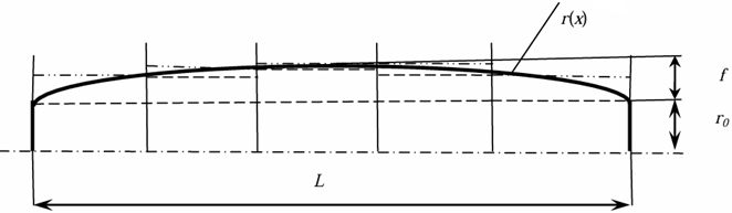
Fig. 7. Inscribed (dashed) and circumscribed (dash–dotted) cylinders for a convex body of revolution

As an illustrative example, a rod is considered whose lateral surface is generated by rotating a sinusoidal curve about the axis:

which possesses the aforementioned properties. The parameter f may take both positive and negative values, thereby defining either a convex profile ( f>0 ) or a concave profile ( f<0 ).

During preliminary computations, it was established that the procedure for estimating the critical load described in Section 2.3, when applied to the rod shown in Fig. 7, converges more slowly than in the case of a conical rod. Specifically, as seen in Table 1, an approximation with 20 discretization elements already yields a relative interval of 0.035 of the mean value, whereas achieving a comparable interval on the order of 0.01 requires approximately 200 subdivisions.

Table 2 presents an estimate of the critical load for the rod in Fig. 7 under various boundary conditions and for different values of the parameter f (note that negative values correspond to a concave profile).

Table 2. Estimation of the critical load for the rod shown in Fig. 5 under various boundary conditions with discretization into 198 segments

Note: The following notation for boundary conditions is used in the table: Z – fixed (clamped) end, S – hinged (pinned) support, F – free end. The first letter corresponds to the beginning of the rod, and the second to its end.

From Table 2, it can be seen that the convergence of the estimation procedure depends on the absolute value of the relative excess of the mean radius over the minimum radius. When this parameter is doubled, the relative interval for determining the critical load $\delta$ also approximately doubles for all boundary condition schemes. The lower and upper estimates of the critical load increase monotonically with increasing parameterf, which is consistent with the intuitive understanding of the stability loss of a composite rod. According to this concept, the critical load is governed by the least stiff element in the system (see, for example, Fig. 3). The achieved level of error (on the order of 0.01–0.03) is quite satisfactory for practical applications. The proposed procedure for determining the critical load is universal with respect to both boundary conditions and the nature of the problem (dead or follower load).

The algorithm is straightforward to implement using general-purpose mathematical software packages; in particular, Mathcad was used in this study. At the same time, the proposed procedure is fully portable to high-level programming environments such as MATLAB or Python, since the formulation is based primarily on recursive matrix operations and standard eigenvalue analysis. This portability makes the method attractive for integration into automated design, optimization, and uncertainty-analysis workflows for structural systems with variable stiffness.

Compared with standard FEM approaches, the proposed IPM formulation avoids complex meshing procedures and relies primarily on recursive transfer-matrix operations with fixed-size matrices. The computational effort increases approximately linearly with the number of discretization segments, which makes the method suitable for refined parametric studies of rods with variable stiffness. In contrast to conventional FEM formulations, the proposed approach does not require repeated global mesh generation or assembly of large sparse stiffness matrices for each geometric configuration. Therefore, the method is computationally convenient for automated design studies and repeated evaluation of variable-stiffness rod models.

4             Conclusions

In this study, the method of initial parameters has been shown to provide a computationally convenient framework for the analysis of centrally compressed rods with variable stiffness. The proposed approach enables the evaluation of critical loads while accounting for the influence and spatial variation of axial forces, without requiring closed-form solutions of differential equations with variable coefficients.

The method applies to both stepped and continuously varying rods, providing reliable upper and lower bounds for critical loads in conservative and non-conservative problems under various boundary conditions. Numerical results demonstrate monotonic convergence of the estimates, with relative deviations below 1–3% for sufficiently refined discretizations. The approach applies to both conservative and non-conservative problems under various boundary conditions, confirming its versatility for stability analysis of structural elements with variable stiffness.

The present approach is limited to linear elastic rod theory and small deformations. In addition, rods with rapidly varying cross-sections may require a relatively large number of segments to obtain narrow estimation intervals. Future work may include extending the proposed approach to nonlinear material behavior, time-dependent loading, and more complex structural systems.

This research is supported by Ho Chi Minh City University of Technology and Engineering (HCMUTE), Vietnam.

The authors declare that there is no conflict of interest regarding the publication of this paper.

Both authors contributed equally to preparing this article.

There is no dataset associated with this study.

There are no supplementary materials to include.

References

- Demidovich, B. P. (1967). Lectures on the mathematical theory of stability. Nauka.
- Babakov, I. M. (2004). Theory of vibrations. Drofa.
- Bolotin, V. V. (1961). Nonconservative problems of the theory of elastic stability. State Publishing House for Physical and Mathematical Literature.
- Volmir, A. S. (1957). Stability of deformable systems. Nauka.
- Gryazev, M. V. (2011). Applied problems of mechanics of deformable solids. Part 1: Statics of rods. Tula State University Publishing House.
- Tolokonnikov, L. A. (1979). Mechanics of deformable solids. Vysshaya Shkola.
- Pavlovskii, M. A., Chemeris, A. N., & Didkovskii, V. S. (1982). Initial-parameter method for bending oscillations of beams with hinges and oscillators. Strength of Materials, 14, 1713–1715. https://doi.org/10.1007/BF00768664
- Hoang, T. T. M., & Le, T. T. (2025). Dynamic analysis of centrally compressed inhomogeneous rods using the initial parameters method. International Journal of Applied Mechanics and Engineering, 30(4), 52–66. https://doi.org/10.59441/ijame/210541
- Yang, L., Yang, B., Yang, G., Xiao, S., Zhu, T., & Jiang, S. (2022). Critical-load calculation method of bolt competitive failure under composite excitation. International Journal of Fatigue, 156, 106660. https://doi.org/10.1016/j.ijfatigue.2021.106660
- Skrinar, M. (2008). On critical buckling load estimation for slender transversely cracked beam-columns by the application of a simple computational model. Computational Materials Science, 43(1), 190–198. https://doi.org/10.1016/j.commatsci.2007.07.029
- Bilgehan, M. (2011). Comparison of ANFIS and NN models—With a study in critical buckling load estimation. Applied Soft Computing, 11(4), 3779–3791. https://doi.org/10.1016/j.asoc.2011.02.011
- Bo, R., & Li, F. (2011). Efficient estimation of critical load levels using variable substitution method. IEEE Transactions on Power Systems, 26(4), 2472–2482. https://doi.org/10.1109/TPWRS.2011.2112782
- Gendy, A. S., & Marzouk, S. S. (2020). Enhanced model including moment-rotation dependency for stability of thin-walled structures. International Journal for Computational Methods in Engineering Science and Mechanics, 21(2), 73–95. https://doi.org/10.1080/15502287.2020.1729897
- Tang, L., Man, X., Zhang, X., Bhattacharya, S., Cong, S., & Ling, X. (2021). Estimation of the critical buckling load of pile foundations during soil liquefaction. Soil Dynamics and Earthquake Engineering, 146, 106761. https://doi.org/10.1016/j.soildyn.2021.106761
- Carpinteri, A., Kurek, M., Łagoda, T., & Vantadori, S. (2017). Estimation of fatigue life under multiaxial loading by varying the critical plane orientation. International Journal of Fatigue, 100(2), 512–520. https://doi.org/10.1016/j.ijfatigue.2016.10.028
- Awrejcewicz, J., Krysko, A. V., Papkova, I. V., Vygodchikova, I. Y., & Krysko, V. A. (2015). On the methods of critical load estimation of spherical circle axially symmetrical shells. Thin-Walled Structures, 94, 293–301. https://doi.org/10.1016/j.tws.2015.04.003
- Huang, Y., & Li, X. F. (2010). A new approach for free vibration of axially functionally graded beams with non-uniform cross-section. Journal of Sound and Vibration, 329(11), 2291–2303. https://doi.org/10.1016/j.jsv.2009.12.029
- Marcinowski, J., & Sadowski, M. (2024). Application of the Southwell method to determine the critical load of compression rods made of nonlinear materials. Civil and Environmental Engineering Reports, 34(4), 168–184. https://doi.org/10.59440/ceer/194260
- Almet, A. A., Byrne, H. M., Maini, P. K., & Moulton, D. E. (2019). Post-buckling behavior of a growing elastic rod. Journal of Mathematical Biology, 78, 777–814. https://doi.org/10.1007/s00285-018-1292-0
- Brailovski, V., Facchinello, Y., Brummund, M., Petit, Y., & Mac-Thiong, J.-M. (2016). Ti–Ni rods with variable stiffness for spine stabilization: Manufacture and biomechanical evaluation. Shape Memory and Superelasticity, 2, 3–11. https://doi.org/10.1007/s40830-016-0053-4
- Koutsogiannakis, P., Misseroni, D., Bigoni, D., & Dal Corso, F. (2023). Stabilization against gravity and self-tuning of an elastic variable-length rod through an oscillating sliding sleeve. Journal of the Mechanics and Physics of Solids, 181, 105452. https://doi.org/10.1016/j.jmps.2023.105452
- Zhang, Q., Zhao, D., Li, W., Zhang, Y., & Zhao, S. (2025). Multi-helix buckling of a slender compression rod constrained by a cylinder. European Journal of Mechanics A/Solids, 109, 105456. https://doi.org/10.1016/j.euromechsol.2024.105456
- Gross, O., Pinkall, U., & Wahl, M. (2025). Elastic curves with variable bending stiffness. Studies in Applied Mathematics, 155(2), e70097. https://doi.org/10.1111/sapm.70097
- Penna, R., Lovisi, G., & Feo, L. (2024). Buckling analysis of functionally graded nanobeams via surface stress-driven model. International Journal of Engineering Science, 205, 104148. https://doi.org/10.1016/j.ijengsci.2024.104148
- Tang, Y., Bian, P.-L., & Qing, H. (2024). Buckling and vibration analysis of axially functionally graded nanobeam based on two-phase local/nonlocal models. Thin-Walled Structures, 202, 112162. https://doi.org/10.1016/j.tws.2024.112162
- Murín, J., Kugler, S., Paulech, J. (2025). Elastostatic analysis of tapered FGM beams with spatially varying material properties. Composites Part C: Open Access, 17, 100592. https://doi.org/10.1016/j.jcomc.2025.100592
- Akhmediev, S., Tazhenova, G. M., Bakirov, M., Filippova, T., & Tokanov, D. (2023). Calculating a beam of variable section lying on an elastic foundation. Journal of Applied Engineering Science, 21(1), 87–93. https://doi.org/10.5937/jaes0-38800
- Lu, J., Xu, L., Xu, H., Li, K., & Hu, J. (2023). Buckling analysis of variable-stiffness composite truncated elliptical rotary shell under external hydrostatic compression. Composite Structures, 307, 116613.
- Akbarova, S. B., & Akhundzada, S. L. (2024). Construction of an inhomogeneous solution for the problem of torsion of a radially inhomogeneous transversal isotropic cylinder. UNEC Journal of Engineering and Applied Sciences, 4(1), 37–72. https://doi.org/10.61640/ujeas.2024.0503
- Ertunç, K., Dilmac, H., & Sofiyev, A. H. (2025). Investigation of stability behavior of clamped functionally graded cylindrical shells in elastic medium under lateral pressure. UNEC Journal of Engineering and Applied Sciences, 5(1), 5–15. https://doi.org/10.61640/ujeas.2025.0501
Conflict of Interest Statement