Original Scientific Paper, Volume 23, Number 2, Year 2025, No 1270, pp 253-268
Received: Oct 30, 2024 Accepted: May 23, 2025 Published: Jun 16, 2025
DOI: 10.5937/jaes0-54461
NUMERICAL ANALYSIS AND SCALED-DOWN MODEL OF AIR BARRIER AND BLOCKING ANGLE VARIATIONS IN SUPPLY DUCT DIFFUSER IN HIGH-SPEED TRAIN CABINS TO COMPLY WITH INDONESIAN THERMAL COMFORT
Abstract
Kereta Cepat Merah Putih (KCMP) was a high-speed train developed by the Indonesian government to enhance intercity travel. A key focus of this development was the HVAC system within the passenger cabin, essential for ensuring passenger comfort. This study investigated the impact of air barrier placement and air flow direction angles (45°, 90°, and 135°) on airspeed and temperature distribution in the cabin. Using CFD simulations with ANSYS Fluent, six variations were tested to determine the optimal configuration. The results identified variation model 3, which employed an air barrier at the top of the ducting system and omitted the use of blocking angles for the air flow direction of the supply diffuser, as the most effective in achieving optimal airspeed and temperature distribution. Following the simulation, experimental measurements were conducted on a scaled-down model of variation 3. Measurements were taken at six sample planes in the supply duct and five in the supply duct diffuser, applying the duct traversing method (ISO 3966) with 25 measurement points per sample plane. The experimental results were then compared with the simulation data to ensure consistency in volumetric flow rate, flow velocity, and air pressure drop parameters. Additionally, comparisons were made with similar trains, measuring air velocity and temperature distribution within their passenger cabins. The findings confirmed that the performance of variation model 3 in the CFD simulation aligned with the scaled-down experimental results, demonstrating consistency in both tests and comparisons.
Highlights
- This study investigated the impact of air barrier placement and air flow direction angles on air velocity and temperature distribution in the KCMP cabin using CFD simulation.
- Variation of Model 3, with an air barrier at the top and no blocking angles, achieved optimal air velocity and temperature distribution.
- Experimental tests on a scaled-down model confirmed the CFD results, validating air velocity, flow rate, and pressure.
Nomenclature
|
|
Cp - Specific heat, J/kg.K |
|
t ̅ - Average temperature, °C |
|
|
k - Thermal conductivity, W/m.K |
|
v ̅ - Average velocity, m/s |
|
|
Kt - Temperature non-uniformity indices |
|
ρ - Density of the material, kg/m3 |
|
|
Kv - Velocity non-uniformity indices |
|
δt - Standard deviation of the air temperature, °C |
|
|
t - Thickness, m |
|
δv - Standard deviation of the air velocity, m/s |
Keywords
Content
1 Inroduction
The Kereta Cepat Merah Putih (KCMP) is a high-speed train being developed by the Indonesian government along the 154 km Makassar–Parepare route. A key component of this system is the HVAC unit in passenger cabins, which ensures thermal comfort defined as the balance between metabolic heat and environmental heat loss [1]. Thermal comfort is achieved when air temperature, humidity, airflow, and radiant heat are within acceptable ranges [2]. Passenger-generated heat significantly affects cabin temperature, requiring efficient thermal control [3]. Due to space constraints and fluctuating passenger loads, a compact and optimized ducting design is essential [4].
Several studies have analyzed airflow and HVAC performance in high-speed trains using Computational Fluid Dynamics (CFD). Yang et al. (2024) examined how diffuser types influence airflow and contaminant transport, highlighting the role of diffuser design in achieving thermal uniformity [5]. Suárez et al. (2017) conducted a parametric CFD study on air distribution in railway vehicles, noting variations in airflow under different weather and operating conditions [6].
Although these studies offer valuable insights, they mainly focus on systems implemented in temperate regions. There is still a lack of research addressing HVAC performance in tropical environments, especially within the framework of local regulatory standards. In Indonesia, thermal comfort standards for high-speed trains are set by the Minister of Transportation Regulation No. 69 of 2019, which specifies an operational temperature range of 22–26 °C and a maximum airspeed of 0.5 m/s [7]. Considering the high energy demands of HVAC systems, optimizing their design is essential for improving energy efficiency and ensuring long-term sustainability. Key indicators of passenger comfort include maximum air velocity, average cabin temperature, and the degree of temperature variation within the space [8].
This research is a continuation of a previous study [9] that focused on optimizing air distribution in diesel-electric multiple unit (DEMU) train cabins. In 2023, the KCMP project switched to using electric multiple unit (EMU) technology, which required a redesign of the HVAC duct layout due to changes in component positions, space availability, and operational heat loads. To address these new design challenges, this study conducted a numerical investigation of the airflow distribution within the KCMP HVAC duct system for the executive, sleeper, and driver cabins. Six configurations were analyzed, involving combinations of air barrier placement (none, top, bottom) and air divider angles (45°, 90°, and 135°). The most promising configuration was then validated through experimental testing using a scaled physical model. This combined simulation-experimental approach aims to inform the design of efficient and climate-appropriate HVAC systems for high-speed rail applications in Southeast Asia.
2 Materials and methods
2.1 Geometry
The interior geometry of the high-speed train cabin in this study is based on a CAD (Computer-Aided Design) drawing from an Indonesian railway vehicle manufacturing company. The design represents an EMU (Electric Multiple Unit) train, specifically the Trailer Car (TC) configuration, which is a passenger car without a propulsion motor system. The model measures 25.3 meter in length, 3.1 meter in width, and 2.1 meter in height. Each carriage is designated to have driver's cabin, sleeper passenger cabin, bathroom/lavatory, economy passenger cabin, and compartment housing the panel box, however in order to simplify the computational process due to the large number of elements generated during meshing, geometric model simplification was performed by removing cabins without passengers. The resulting simplified geometry is shown in Figures 1.

Fig. 1. Isometric view of 3D model geometry of Kereta Cepat Merah Putih (KCMP) after simplification
2.2 Variations of air barrier and supply diffuser air flow direction blocking angle
The ducting systems in this study consists of 2 supply ducts, each with 8 supply diffusers and 8 air barriers, and 1 return duct without an air barrier, as illustrated in Figure 2. The research began with a baseline design (Variation 1) using ducting without an air barrier. Subsequent designs incorporated air barriers at the bottom (Variation 2) and top (Variation 3) of the ducting to evaluate their impact on temperature and airspeed distribution. In addition to simulating air barrier variations, simulations were also conducted on different blocking angles for the supply diffuser's air flow direction. Three angles were tested: 45°, 90°, and 135°. The most optimal results from the air barrier variations will be combined with the blocking angle variations to achieve the best ducting design. Details on air barrier dan the blocking angles for the supply diffuser air flow can be seen in Figure 3.
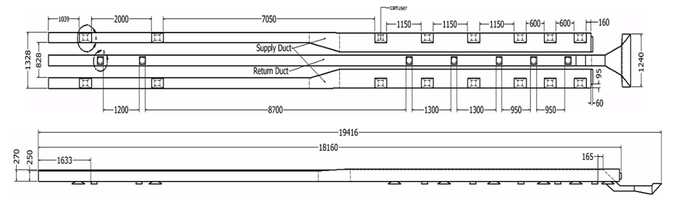
Fig. 2. Top and side view of ducting systems
|
(a) |
(b) |
(c) |
|
(d) |
(e) |
(f) |
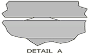
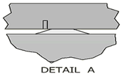
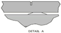
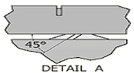
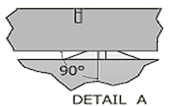
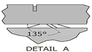
Fig. 3. Details of the air barrier position and diffuser supply air flow direction blocking angle: (a) variations 1, (b) variations 2, (c) variations 3, (d) variation 4, (e) variations 5, and (f) variations 6
Therefore, based on the provided explanation, there are a total of six variation models, focusing on variations in the use of air barriers and the blocking angles for the air flow direction of the supply diffuser in the train passenger cabin. The detailed descriptions of these variations are summarized in Table 1.
Table 1. Variations of air barrier configuration scheme and air flow direction blocking angle of supply diffuser
| Variations | Air Barrier | Diffuser Supply Air Flow Direction Blocking Angle |
| 1 | Ducting System Without Using Air Barrier | Omitting the use of blocking angles for the air flow direction of the supply diffuser |
| 2 | Using an air barrier at the bottom | |
| 3 | Using an air barrier at the top | |
| 4 | Blocking angle of 45° | |
| 5 | Blocking angle of 90° | |
| 6 | Blocking angle of 135° |
2.3 Meshing
Meshing transforms a model's geometric domain into smaller discrete elements or nodes, allowing the continuous fluid domain to be discretized into a computational domain solvable by CFD software. In this case, meshing was conducted with sizes of 12 mm for human elements, 100 mm for walls, 48.5 mm for side and front windows, and 45 mm for inlets and outlets. This produced approximately 15,647,141 elements and 2,981,378 nodes, with average skewness and orthogonal quality values of 0.22971 and 0.76893, respectively—both within the acceptable range according to ANSYS 2013 standards. The geometric results of the mesh model are shown in Figure 4.
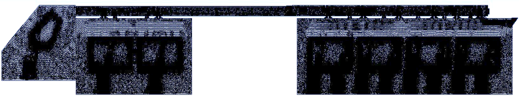
Fig. 4. Mesh display of geometric models
2.4 Setup, boundary conditions and material parameters
CFD simulation of the model was carried out using ANSYS Fluent software. The simulation setup is conditioned in steady state conditions with the SIMPLEC method solution. In this study, air flows from an air conditioner with a cooling capacity of 35 kW and a volumetric flow rate of 3000 m3/h, which is then converted into mass flow inlet parameters [9]. Additionally, boundary condition settings were applied to the outlet, walls, window seats, passengers, and other parameters derived from calculations and literature studies conducted. More detailed information regarding the simulation setup used and the boundary condition settings can be seen in Table 2.
Table 2 (a). Details of simulation setup settings and boundary condition
| Simulation Setup Settings | |||
| General | Solver | Type | Pressure-based |
| Time | Steady | ||
| Gravity | Acceleration | Y = -9.81 m/s2 | |
| Model | Energy | On | |
| Viscous | K-epsilon realizable | Standard wall function | |
Table 2 (b). Details of simulation setup settings and boundary condition
| Solution Method | Pressure velocity-coupling | Scheme | SIMPLEC | ||
| Spatial discretization | Gradient | Least Square cell based | |||
| Pressure | Second order | ||||
| Momentum Turbulent kinetic energy, turbulent dissipation rate, Energy | Second order upwind | ||||
| Boundary Conditions | |||||
| Inlet | Mass Flow Inlet (1 kg/s) | Floor | Adiabatic | ||
| Temperature: 20°C | Front Window | Convection: 4.56 W/m2.K | |||
| Outlet | Pressure-outlet | Free stream temperature: 30°C | |||
| Gauge pressure: 0 Pa | Side Window | Convection: 1.8 W/m2.K | |||
| Wall | Adiabatic | Free stream temperature: 30° C | |||
| Seat | Adiabatic | Passenger | Temperature: 37°C | ||
2.5 Mesh independency test and simulation validation
The simulation, guided by relevant equations, relies on a well-structured mesh for accuracy [10]. To predict numerical uncertainty and validate the simulation, a mesh independence test is conducted. This involves running simulations with varying mesh element counts to observe changes in solution convergence. In this study, five mesh variations are tested: 13,533,081; 14,107,818; 14,723,175; 15,293,194; and 15,897,120 elements. The results, shown in Figure 5, indicate that the average air velocity in the business class passenger cabin stabilizes at 15,293,194 elements. Therefore, subsequent models use at least this many elements.
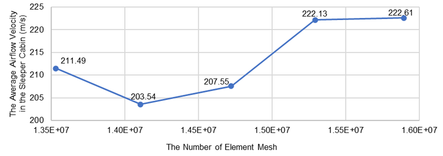
Fig. 5. Mesh independency test
2.6 Air temperature distribution simulation results
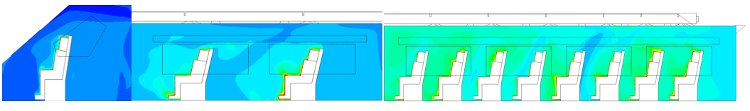
The analysis of temperature distribution begins with observing the temperature volume rendering in each cabin across various model variations. For example, Figure 6 presents the temperature volume rendering for model variation 1. It is clear from the figure that both the economy and sleeper cabins have an average air temperature between 22-24°C, as indicated by the transition from light green to dark green. In contrast, the driver's cabin is depicted in a darker blue color, reflecting lower temperatures ranging from 20 to 21.6°C. For a clearer understanding of the average air temperature distribution, the exact average temperatures for each cabin in all model variations are detailed in Table 3.
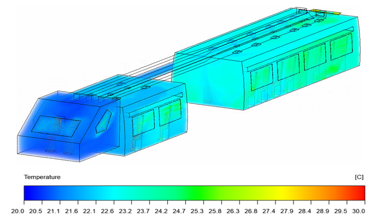
Fig. 6. Isometric view of the volume rendering of air temperature for variation 1
Tabel 3. Average air temperature data in each cabin all variation models
| Variation Model | Average Air Temperature (°C) | ||
| Economy Cabin | Sleeper Cabin | Driver Cabin | |
| 1 | 23.51 | 22.54 | 21.50 |
| 2 | 23.79 | 23.38 | 22.08 |
| 3 | 23.63 | 22.96 | 22.20 |
| 4 | 23.71 | 22.87 | 22.09 |
| 5 | 23.62 | 22.86 | 22.05 |
| 6 | 24.07 | 22.79 | 21.83 |
Based on the table, it is clear that several model variations do not meet the established thermal comfort standards. In the comparison of model variations using air barriers, the average air temperature in the driver's cabin for model variation 1 does not meet the thermal comfort standard, remaining below the 22–26°C range, when compared to model variations 2 and 3. Similarly, in the comparison of model variations using deflector angles, the average air temperature in the driver's cabin for model variation 6 also falls short of the thermal comfort standard, compared to model variations 4 and 5. To observe the temperature conditions of air flow interacting with passengers, the average temperature data of each passenger column in each cabin was taken. Figure 7 depicts the passenger column of each cabin on this train, and Table 4 is the average temperature data of each passenger column. This is intended to determine the temperature distribution of each passenger column, given the location of the supply duct closer to the center.
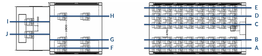
Fig. 7. Passenger column location in each cabin
Tabel 4. Average air temperature data of passenger column all variation models
| Variation Model | Average Air Column Temperature (ºC) | |||||||||
| Driver Cabin | Sleeper Cabin | Economy Cabin | ||||||||
| J | I | H | G | F | E | D | C | B | A | |
| 1 | 20.97 | 20.98 | 22.21 | 22.45 | 22.42 | 23.57 | 23.31 | 23.48 | 23.45 | 23.78 |
| 2 | 21.37 | 21.41 | 22.67 | 22.64 | 22.8 | 23.77 | 23.43 | 23.39 | 23.25 | 23.73 |
| 3 | 21.4 | 21.41 | 22.62 | 22.49 | 22.61 | 23.54 | 23.5 | 23.56 | 23.14 | 23.45 |
| 4 | 21.28 | 21.27 | 22.5 | 22.5 | 22.58 | 23.63 | 23.57 | 23.78 | 23.23 | 23.43 |
| 5 | 21.27 | 21.25 | 22.3 | 22.45 | 22.75 | 23.86 | 23.43 | 23.42 | 23.09 | 23.57 |
| 6 | 21.12 | 21.21 | 22.51 | 22.23 | 22.21 | 24.06 | 23.72 | 23.93 | 23.52 | 23.92 |
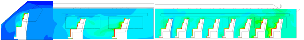
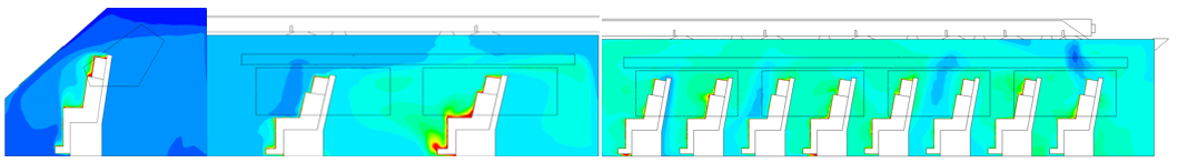
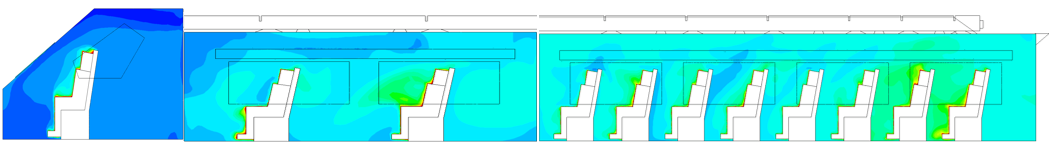
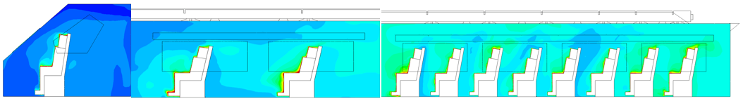
At first glance it appears that the temperature in each passenger column in each cabin is quite well distributed, although in the driver's cabin the temperature is still slightly below the standard. but for economy and sleeper passenger cabins, all variations have shown a fairly good distribution while still meeting thermal comfort temperature standards. the contour feature is also used to see the temperature distribution in one of the passenger columns in each cabin. The selected passenger column is the column closest to the air supply diffuser, namely column B in the economy cabin, column G in the executive cabin, and column J in the driver cabin. Figure 8 presents the temperature contour display for each model variation. Based on the figure, almost all model variations show similar contour colors in each cabin. However, compared to the other model variations, model variation 1 at the rear of the economic cabin has a darker green color, indicating that the airflow in the ducting system in this variation is not well distributed at the rear of the cabin, resulting in higher temperature values.
 |
(1) |
 |
(2) |
 |
(3) |
 |
Fig. 8 (a). Air temperature contour of passenger column variations
 |
(4) |
 |
(5) |
 |
(6) |
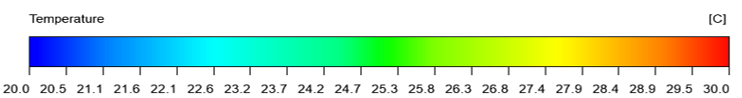 |
Fig. 8 (b). Air temperature contour of passenger column variations
2.7 Air velocity distribution simulation results
Similarly, the process of reviewing the airflow distribution for each cabin in all model variations also uses the volume rendering feature, as shown in Figure 9, which is the volume rendering of the air velocity for variation 1. In the ducting system, especially in the supply duct section in the economy cabin, the dark red color indicates that the airflow in this section has a maximum velocity in the range of 4.2 - 5.0 m/s. This is because the airflow is still close to the inlet. Then, the airflow in the ducting system towards the passenger and driver cabins appears light green in color, indicating a decrease in speed in the range of 1.8 - 2.6 m/s. In addition, the visualization of the color change from dark red to light blue is also seen in the supply diffuser section which shows the maximum airflow velocity when entering the passenger cabin, which then decreases as it approaches the passenger area.
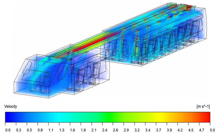
Fig. 9. Isometric view of the volume rendering of air velocity for variation 1
It should be noted that the maximum air velocity of 0.5 m/s referred to in the ministry of transportation regulation number 69 of 2019 above, is the maximum limit of air velocity received by passengers at a height of 1.2 m from the floor as a representation of the passenger's head position in a sitting state, which means it is not the average air velocity in the cabin. Therefore, in addition to volume rendering, velocity vector data was collected for all model variations to analyze the airflow movement from the supply duct to each passenger cabin. Figure 10 shows that air flow velocity is generally higher in the ducting channels and lower in the passenger cabin areas. In model variation 1, the supply diffuser near the AC air inlet duct is bypassed by air flow due to the absence of an air barrier component to redirect the high-velocity air into the cabin. The use of deflector angles, as seen in variations 4, 5, and 6, also affects the uniform distribution of air flow within the passenger cabin.
|
(1) |
(2) |
|
(3) |
(4) |
|
(5) |
(6) |
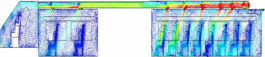

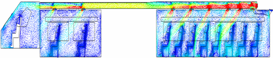
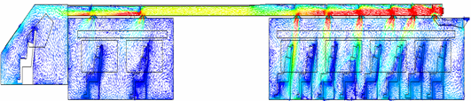
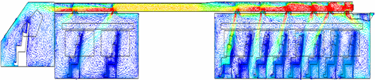

Fig. 10. Air velocity vector of supply air diffuser flow and train passenger cabin variations
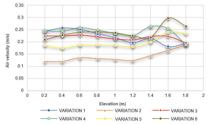
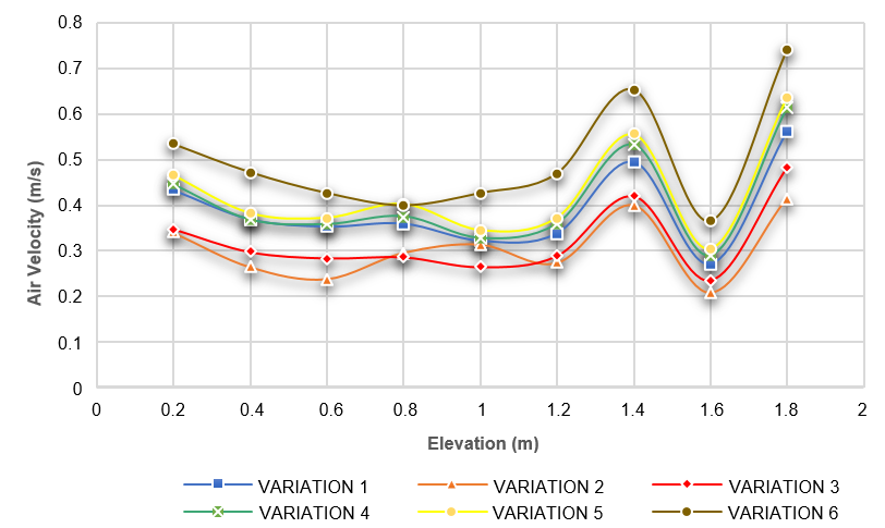
To review in more detail, Figure 11 presents three graphs comparing the simulation results of different model variations by analyzing the vertical distribution of the average air velocity in each passenger cabin of the train. The graphs show that at heights between 0.2 and 1 meter, the average air velocity decreases slightly, followed by a significant increase between 1.2 and 1.8 meter, where the air supply is closer to the diffuser. On this train, passengers are seated in the height range of 0 to 1.4 cm, where in that height range the average air velocity meets the requirements. Although, there are some variations, especially in the economy cabin, which still exceed the requirements, this is due to the large number of diffusers in the cabin.
![]()
(a)
(b)
(c)
Fig. 11. The curve of comparison for the distribution of average surface velocity across all variations
(a) economy cabin, (b) sleeper cabin, (c) driver cabin.
2.8 Temperature and velocity nonuniformity indices (TNUI and VNUI)
The thermal comfort of a passenger is evident in the non-uniformity of air temperature distribution within the train's passenger cabin area. A smaller non-uniformity index value indicates a more favorable uniformity in air temperature distribution throughout the cabin. The calculation of temperature non-uniformity indices can be derived from Equation 1[11].
 |
(1) |
The standard deviation of air temperature around the passenger, denoted as and the average temperature of all measured points were analyzed. This study measured 48 sample points around the passenger area to assess temperature uniformity. These points were located 20 mm in front of each passenger's head and 1.2 meter above the floor.
As illustrated in Figure 12, Variation 6, which applies a ducting system with air barriers at the top and a 135° blocking angle for the supply diffuser air flow, shows the highest temperature non-uniformity index. In contrast, Variation 3, which has air barriers but no blocking angle, results in the lowest index.
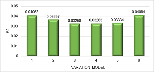
Fig. 12. Graphic of air temperature nonuniformity index (TNUI)
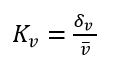
Similar to air temperature parameters, an analysis of airspeed parameters can also be conducted using the calculation of non-uniformity index values. A lower non-uniformity index value signifies a more uniform distribution of airspeed in the cabin. The calculation of velocity non-uniformity indices can be obtained using Equation 2.
 |
(2) |
The standard deviation of air velocity around passengers and the average velocity across all measured points were analyzed. The study measured 48 sample points around each passenger to assess the uniformity of air velocity, with points located 20 mm in front of the passenger’s head and 1.2 meter above the floor.
According to Figure 13, Variation 6, which applies a ducting system with air barriers at the top and a 135° blocking angle for the supply diffuser air flow, shows the highest velocity non-uniformity index. In contrast, Variation 3, which has air barriers but no blocking angle, results in the lowest index.

Fig. 13. Graphic of air velocity nonuniformity index (VNUI)
So, Variation 3 was chosen to be the best variation among the other six variations. The study continued by further analyzing the supply duct of this variation.
3 Results and discussion
3.1 Analysis of selected supply duct through simulation
Once the optimal duct geometry, identified as variation 3, has been established to ensure thermal comfort for passengers on the train, a more comprehensive analysis of the airflow within the supply duct is conducted. The purpose of this analysis is to determine the flow pattern and pressure drop in the duct. In general, the velocity vector of the air flow in the supply duct can be seen in Figure 14.

(a)
![]()
(b)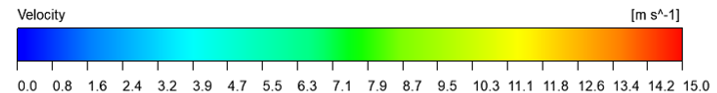
Fig. 14. Air velocity vector in (a) front duct segment, dan (b) transition duct segment dan rear duct segment
An examination of the air flow velocity vector image reveals a decrease in flow velocity along the channel, with higher velocity observed near the inlet. This phenomenon is consistent with the principles set forth by Bernoulli, which state that as flow velocity increases and static pressure decreases through a shrinking duct, the relationship between the two is inversely proportional [12]. Therefore, an increase in velocity is observed at the transition segment, which features a reduced cross-section. Furthermore, the velocity of the flow exiting the diffuser is consistent with the figure, wherein the diffuser in closest proximity to the supply duct inlet exhibits a slower flow rate than the diffuser situated adjacent to it, as indicated by the color differentiation evident in the figure. In order to provide an in-depth explanation of the air flow phenomenon in the supply duct, this study will analyze the static, dynamic and total pressures at each sample plane along the supply duct and diffuser. The plane samples are also the same plane samples used for experimental measurements to validate the simulation. There are a total of 11 plane samples, divided into six plane samples inside the supply duct and five plane samples in the cross-sectional area of the supply duct diffuser. Figure 15 shows a detailed overview of the airflow in each plane sample measurement.

Fig. 15. Detail of air velocity vector at duct plane 1-6
Duct Plane 1 shows a high air flow velocity, as indicated by the high dynamic pressure, which reflects the high velocity at this point. The relatively high total pressure suggests that the energy in the flow is well-maintained at the duct's starting point, likely because this plane is closest to the inlet. Moving to Duct Plane 2, there is a higher static pressure but significantly lower dynamic pressure, indicating a lower flow velocity compared to Duct Plane 1. The substantial drop in dynamic pressure signals a decrease in flow velocity, while the increase in static pressure is likely due to increased resistance from obstacles like air barriers. The velocity vectors in this plane are predominantly green and blue, with fewer 3D arrows compared to Duct Plane 1. Duct Planes 3 through 6 show variations in static and dynamic pressures, but overall, the total pressure decreases along the duct, indicating a pressure drop along the flow path. The total pressure, which is the sum of static and dynamic pressures, decreases throughout the duct and diffuser, reflecting a loss of total energy due to friction, changes in geometry, or flow dissipation.
3.2 Scaled-down measurement of selected supply duct for comparison to simulation
3.2.1 Sample plane on the supply duct
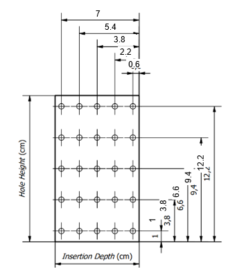
The simulation of the selected supply duct design and the experimental measurements of the scaled-down supply duct are conducted on the same 11 sample planes. The sample planes are divided into two categories: six sample planes located within the supply duct and five sample planes situated on the cross-sectional area of the supply duct diffuser. The scaled-down supply duct has been constructed with a downscaling factor of 1:3 in comparison to the original simulated supply duct design. The specific locations of the 11 sample planes on the supply duct are illustrated in Figure 16.
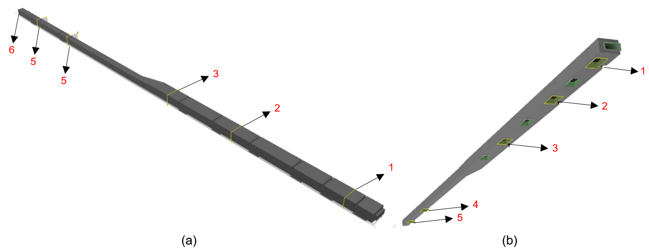
Fig. 16. Detail of sample locations in (a) duct plane 1 to 6, and (b) diffuser plane 1 to 5
3.2.2 Air flow measurement method
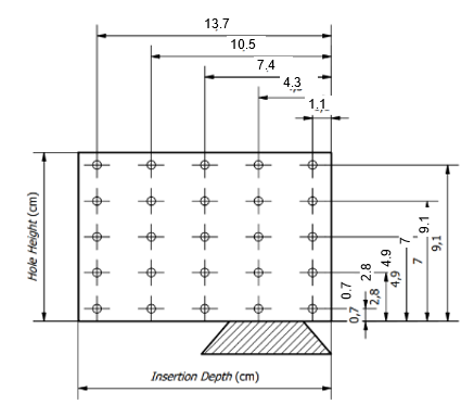
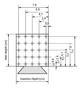
In this study, the duct traversing method (ISO 3966) was employed for experimental measurements. This entailed the identification of 25 measurement points in each sample plane, which were subsequently averaged to yield a representative value. The application of the duct traversing method at both measurement locations is illustrated in the Figure 17.
 |
 |
 |
| Duct Plane 1-3 | Duct Plane 4-6 | Diffuser Plane 1-5 |
Fig. 17. Application of the duct traversing method
The initial stage of the procedure is conducted using a Pitot Tube Anemometer and Manometer, with measurements taken to obtain the volumetric air flow rate and air velocity at the furthest distance for each traversal point [13]. This aligns with the standards set in ISO 3966: 2008. Once the data has been recorded at each point, the mean value of the flow velocity and air pressure at each sample plane is calculated. The measurement process is illustrated in Figure 18.
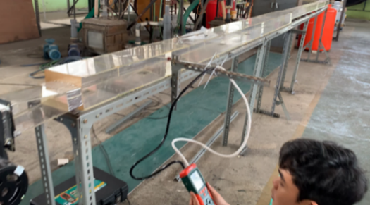
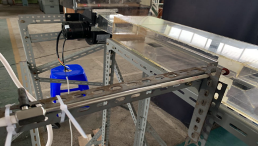
Fig. 18. Experimental measurement setup
3.2.3 Analysis of air flow velocity distribution at each sample plane
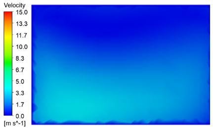
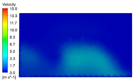
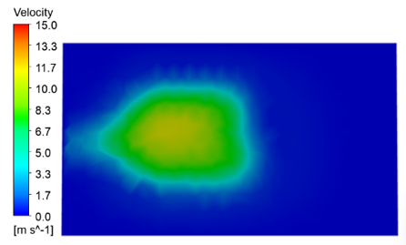
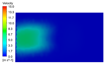
Finally, the velocity distribution on each sample plane is analyzed through the presentation of velocity contours obtained from the simulation results, followed by a comparison with the measured values obtained through the use of experimental methods. The measurement is conducted at 25 points in the sample plane and the resulting value is displayed in a table, with the magnitude of the air flow velocity represented by color. The results of the simulation of the air velocity distribution in relation to the experimental measurement are presented in Figure 19.
| Experimental | Simulation | |||||||||||||||||||||||||||||||||||||||||||||||
| Duct Plane 1 | ||||||||||||||||||||||||||||||||||||||||||||||||
|
 |
|||||||||||||||||||||||||||||||||||||||||||||||
| Duct Plane 3 | ||||||||||||||||||||||||||||||||||||||||||||||||
|
 |
|||||||||||||||||||||||||||||||||||||||||||||||
| Duct Plane 5 | ||||||||||||||||||||||||||||||||||||||||||||||||
|
 |
|||||||||||||||||||||||||||||||||||||||||||||||
| Diffuser Plane 1 | ||||||||||||||||||||||||||||||||||||||||||||||||
|
 |
|||||||||||||||||||||||||||||||||||||||||||||||
| Diffuser Plane 3 | ||||||||||||||||||||||||||||||||||||||||||||||||
|
 |
|||||||||||||||||||||||||||||||||||||||||||||||
|
||||||||||||||||||||||||||||||||||||||||||||||||
|
 |
|||||||||||||||||||||||||||||||||||||||||||||||
The experimental measurements were taken at 25 different points on the sample plane and the results are presented in tabular form, with the color of each cell correlating to the measured air flow velocity. The simulation results provide a continuous contour map of the air flow velocity distribution over the aforementioned plane. The contour map employs color gradients to represent disparate velocity ranges, thus facilitating a visual comparison with the experimental data. A notable correlation was observed between the experimental measurements and the simulation when the two methods were compared. Both methods indicate areas of higher and lower velocity, as indicated by the color codes. The simulation contour map provides a more detailed and continuous representation of the velocity distribution, which may elucidate subtle gradients and variations that are not captured by the discrete 25-point measurement grid employed in the experimental method. The combination of these methods allows for a comprehensive understanding of the air flow characteristics within the sample plane to be achieved.
3.2.4 Comparison of simulation and experimental measurements result on volumetric flow rate
Figure 20 represents the difference between simulation results and experimental measurements obtained from a 1/3-scale supply duct model. At duct plane 1, the simulation indicates a volume flow of 0.325 m³/s, whereas the experimental measurements demonstrate a value of 0.276 m³/s. This pattern persists as the subsequent duct planes are considered. The largest percentage deviation is observed at diffuser plane 2, with a value of 23.63%, while the smallest is seen at diffuser plane 4, with a value of 8.39%. The mean percentage discrepancy between the simulation and experimental outcomes is 15.43%. Both the simulation and the experimental method demonstrate a consistent decline in the flow rate along the diffuser planes.
|
(a) |
(b) |
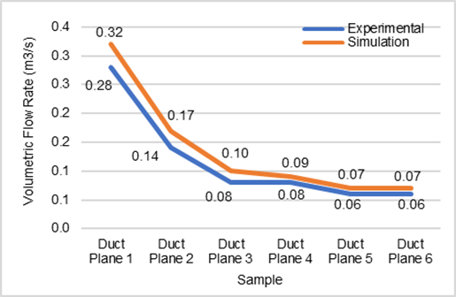
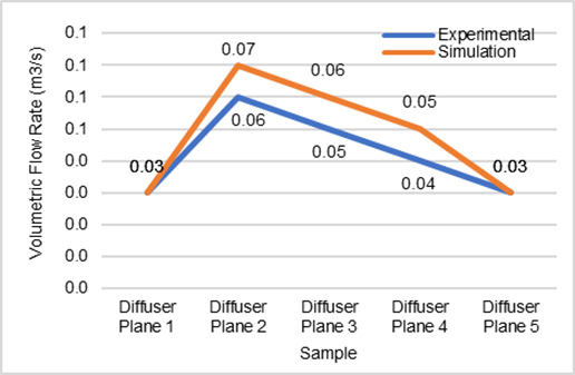
Fig. 20 Volumetric flow rate comparison on (a) duct planes, and (b) diffuser planes
3.2.5 Comparison of simulation and experimental measurements result on air flow velocity
Figure 21 illustrates the discrepancies between the simulation results and the experimental data from the scaled-down supply duct model. At duct plane 1, the simulation shows an air flow velocity of 7.31 m/s, while the experimental measurement is lower at 6.26 m/s. This discrepancy continues across the subsequent duct planes, with varying velocities between the simulation and experimental data. For example, at duct plane 2, the simulation records 3.78 m/s compared to the experimental measurement of 3.18 m/s. The difference is more significant at duct plane 3, where the simulation shows 2.18 m/s and the experimental measurement is 1.91 m/s.
|
(a) |
(b) |
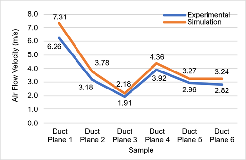
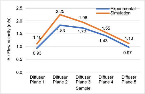
Fig. 21. Air flow velocity comparison on (a) duct planes, and (b) diffuser planes
Similar discrepancies are observed in the diffuser plane section. At diffuser plane 1, the simulation indicates an air velocity of 1.1 m/s, while the experimental measurement is 0.93 m/s. The largest discrepancy occurs at diffuser plane 2, with the simulation at 2.25 m/s and the experimental measurement at 1.83 m/s. The percentage deviation in air velocity at each sample plane mirrors the pattern observed for the flow rate, with an average deviation of 15.16% between the simulation and experimental results. Despite these discrepancies, the overall pattern of air flow velocity variation along the duct and diffuser planes is consistent between the two methods, reflecting the behavior of air flow within the duct system [14].
3.2.6 Comparison of simulation and experimental measurements result on pressure drop
The study focuses on total pressure drop, which better characterizes the air flow pressure drop within the duct. As shown in Figure 22, the air pressure drop is represented by two plane samples taken at duct planes 1 and 6, relative to the pressure at the supply duct inlet. The pressure drops at plane 1 is calculated as the difference between the inlet pressure and the pressure at plane 1. These two planes were chosen because they adequately describe the pressure drop along the supply duct. This discrepancy, 18.64%, can be attributed to the non-linear scaling of physical phenomena in fluid flow. For example, wall friction and turbulence effects may differ at smaller scales, even with the same flow rate. Additionally, static and total pressures are affected by changes in cross-sectional area and wall friction, which do not scale linearly, especially at smaller scales where friction effects are more significant.
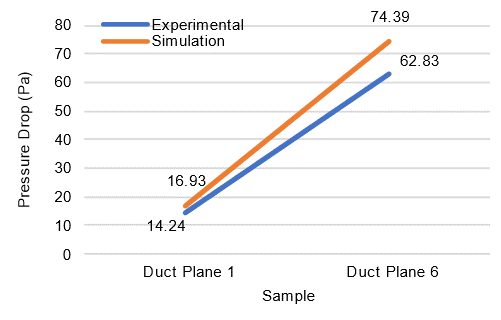
Fig. 22. Pressure drop comparison
3.3 Measurements on operating trains’ s cabin for comparison to simulation
The CFD simulation method for the KCMP passenger cabin was validated by comparing its results with direct measurements taken inside a long-distance executive train passenger cabin. Benchmark data, including temperature and air velocity, were collected using an envirometer at a height of approximately 1.2 meter in front of passengers. These measurements, taken at various points within the cabin, are illustrated in Figure 23. The validation results are presented in Table 5. As shown, the deviation values for both temperature and air velocity are below 5%, which is considered relatively small and acceptable. Therefore, the method used is deemed sufficiently accurate and suitable for representing real conditions in the train passenger cabin.
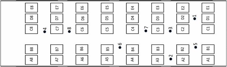
Fig. 23. The location of measurement points inside the train passenger cabin
Once the temperature and air velocity measurement data has been obtained, it is compared with the simulation data. The comparison of both data can be seen in the following table.
Table 5. The air temperature and velocity data from measurements and simulations
| Measurement Points | Air Temperature (ºc) | Air Velocity (ºc) | ||||
| Simulation | Measurement | Error (%) | Simulation | Measurement | Error (%) | |
| A4 | 22.30 | 23.04 | 3.31 | 0.170 | 0.175 | 2.90 |
| B4 | 22.08 | 23.02 | 4.26 | 0.050 | 0.052 | 4.00 |
| C6 | 22.44 | 23.04 | 2.67 | 0.180 | 0.186 | 3.33 |
| D6 | 22.36 | 23.08 | 3.22 | 0.130 | 0.133 | 2.33 |
From the comparison, it is known that the error value of several samples taken does not exceed 5%, so it can be said that the simulation method used is quite appropriate and the design made is good enough.
4 Conclusions
This study analyzes the influence of variations in the use of air barriers and the blocking angles for the air flow direction from the diffuser supply on the distribution of temperature and air velocity inside the train passenger cabin. Based on the conducted research, it can be concluded that:
1. The use and placement of air barriers in the ducting system significantly affect airflow dynamics within both the ducting system and the train passenger cabin. Air barriers play a key role in regulating temperature and air velocity distribution trends, aiming to achieve airflow that meets thermal comfort standards inside the cabin. An analysis of velocity vectors shows that deflector plates used to control airflow direction from the supply diffuser can precisely manage airflow based on the selected deflector angle.
2. Based on a review of the value of the temperature and air velocity non-uniformity index, variation model 3 has the lowest value compared to other variation models, namely 0.03258 for air temperature parameters and 0.5474 for air velocity parameters. This shows that variation model 3 provides the best uniformity of temperature and air velocity values in the passenger cabin area compared to other variation models.
3. Overall, the simulations of the six variation models have not yet met the Indonesian thermal comfort, particularly regarding average air velocity in the train passenger cabin. However, the simulation data indicates that using air barriers and adjusting the blocking angle of the diffuser supply air flow significantly influences temperature and air velocity. Therefore, these components warrant further evaluation.
4. The results show that the volumetric flow rate, flow velocity, and air pressure drop parameters in the selected supply duct design align with the scaled-down model, despite deviations of 15.43% for volumetric flow rate, 15.16% for flow velocity, and 18.64% for pressure drop. This suggests that the scaled-down model is effective for improving and validating simulation models, though slight deviations should be considered. The model offers valuable insights into airflow behavior within ducting systems.
Acknowledgements
This research was the result of a project entitled Pengembangan dan Pembuatan Kereta Cepat Merah Putih (KCMP) Tahap III with the grant number of 142/E1/KS.00.00/2024 which was funded by Kedaireka Program Dana Padanan (PDP), Ministry of Education, Culture, Research, and Technology Indonesia, Year 2024 Batch 3.
References
- SARNA, I., PALMOWSKA, A. (2019). MODELLING OF THE AIR FLOW IN THE PASSENGER COACH. Architecture Civil Engineering Environment Journal, vol. 12, no. 4, 125-133, DOI: 10.21307/ACEE-2019-058.
- Haller, G. (2006). Thermal Comfort in Rail Vehicles. RTA Rail Tec Arsenal Fahrzeugversuchsanlage GmbH, Vienna.
- Rugh, P., Bharathan, D. (2005). Predicting Human Thermal Comfort in Automobiles. SAE Technical Papers 2005-01-2008, 11, DOI: 10.4271/2005-01-2008.
- Min, A., Fan, Y., Wei, H., Zhang, L., Jing, L., Han, Y., Yu, F. (2017). Numerical Study on Aerodynamic Characteristics of High-Speed Trains with Considering Thermal-Flow Coupling Effects. Journal of Vibroengineering, vol. 19, no. 7, 5606-5626, DOI: 10.21595/jve.2017.18778.
- Yang, Lin. Li, Mengxi. Li, Xiangdong. and Tu, Jiyuan. (2024). The Effects of Diffuser Type on Thermal Flow and Contaminant Transport in High-Speed Train (HST) Cabins – A Numerical Study. International Journal of Ventilation, vol. 17, no. 1, 48-62, DOI: 10.1080/14733315.2017.1351736
- Suárez, C., Iranzo, A., Salva, J. A., Tapia, E., Barea, G., & Guerra, J. (2017). Parametric Investigation Using Computational Fluid Dynamics of the HVAC Air Distribution in a Railway Vehicle for Representative Weather and Operating Conditions. Energies, vol. 10, no.8, 1074. DOI: 10.3390/en10081074
- Menteri Perhubungan RI (2019). Peraturan Menteri Perhubungan Republik Indonesia Nomor PM 69 Tahun 2019 Tentang Standar Spesifikasi Teknis Kereta Api Kecepatan Tinggi. Kementerian Perhubungan Republik Indonesia, Jakarta.
- Selamat, H., Fadzli, M., Mat, Z., Mohammad, S., Mohd, F., Al’Hapis, M. (2020). Review on HVAC System Optimization Towards Energy Saving Building Operation. International Energy Journal. vol. 20, no. 3. 345-358.
- Fauzun, F., Yogiswara, C. W., Ariyadi, H. M., Taufiqurrahman, M. S., Ritonga, A. F., Pranoto, I., Garingging, R. A., Areli, F., Putra, R. K., Al-Qadri, M. H., Fatkhi, A. S., Nurdiansyah, R. T., & Restu, F. R. (2023). Numerical Study the Effect of Air Barriers Height Inside the Air Conditioning Ducting to Satisfy the Regulation of Indonesia Minister of Transportation Number 69 Of 2019. Journal of Applied Engineering Science, vol. 21, no. 4, 1156–1170, DOI: 10.5937/jaes0-45415.
- Incropera, F. P., DeWitt, D. P., Bergman, T. L., Lavine, A. S. (2006). Fundamentals of Heat and Mass Transfer Sixth Edition. McGraw-Hill, New York.
- Seeni, A., Rajendran, P., Mamat, H. (2019). A CFD Mesh Independent Solution Technique for Low Reynolds Number Propeller. CFD Letters Journal, vol. 11, no. 10, 15-30.
- Cengel, Y., Cimbala, J. (2015). Fluid Mechanics: Fundamental and Applications. McGraw-Hill, New York.
- Caré, I., Bonthoux, F., Fontaine, J. (2014). Measurement of Air Flow in Duct by Velocity Measurements. EPJ Web of Conferences, vol. 77. 16th International Congress of Metrology, DOI: 10.1051/epjconf/20147700010.
- Li, C., Herrin, D. (2022). Scaled Down Measurement of HVAC Duct Insertion Loss and Comparison to Simulation. INTER-NOISE and NOISE-CON Congress and Conference Proceedings, vol. 264, no. 1, 909–916. DOI: 10.3397/nc-2022-834.
Conflict of Interest Statement
The authors declare that there is no conflict of interest in this research.
Author Contributions
Data Availability Statement
The research data are available from the corresponding author upon reasonable request via email (fauzun71@ugm.ac.id), provided a valid scientific justification is given.
Supplementary Materials
There are no supplementary materials to include.